Guide
The material that used to live in the README, at full length: the model, the scenarios, drawing, planning, and how to reproduce the reported experiments.
The model
| State | DuckieWorldState — the full latent world: delayed DB18 motor model, duckie objects, stop memory, map. Branchable, so a generative planner can copy it safely. |
| Actions | 7 macro actions (FAST_LEFT … BRAKE), or a continuous DuckieAction(v, ω) box |
| Reward | lane progress, lateral and heading error, stop-sign compliance, pedestrian yielding, stagnation, steering smoothness |
| Termination | off-road, collision, duck collision, timeout |
| Discount | 0.99 |
Two projections of the latent state are what policies actually consume:
RawState— 7 components, discretized for tabular methodsContinuousState— 15 components, the encoding SAC/TD3 were trained on
raw, _ = get_raw_state(s, mdp.transition.state_cfg)
raw.d, raw.phi        # lateral offset (m), heading error (rad)
discretize(raw)       # the tabular index
Both are privileged: they are read out of the latent world, not estimated from sensors. Only 6 of the 15 continuous components are sensor-estimable and 2 are agent memory with no physical counterpart at all, so this is a decision-making benchmark and not a perception one. There is deliberately no observation or belief layer.
Scenarios
scenario_config builds a complete world with no external file:
scenario_config(:stop_and_duck)                      # a stop sign, and a duck that crosses
scenario_config(:lane_following)                     # the Python source defaults
scenario_config(:stop_and_duck; algorithm = :td3)    # for the continuous action space
default_config(:q_learning) returns the Python source defaults directly. Be aware of what that world contains: no stop sign at all, and a duck that crosses on 2 % of episodes. It exists for provenance checks, not for driving.
A worked example
examples/quickstart.jl runs end to end with nothing installed but the package itself. It builds a world, rolls out a hand-written lane follower against an always-straight baseline, inspects the privileged projections, and pulls the scene geometry out with no plotting backend present. Same content as a notebook: examples/quickstart.ipynb.
julia --project=. examples/quickstart.jlThe notebook is generated from the script by tools/make_notebook.jl, and CI fails if the two drift apart.
Drawing things
All scene geometry is computed in the core and is inspectable with no plotting package installed; a backend only draws it.
scene = world_scene(mdp, s)     # tiles, lane centrelines, footprint, stop lines
scene.stop_lines                # available with no Makie installed

using CairoMakie                # now the renderers exist
save("world.png", render_world(mdp, s))render_world, render_projection, render_policy, render_search, render_rollout, render_diagnostics, render_animation and render_composite all appear once Makie is loaded. render_observation and render_belief are deliberately not implemented — those signatures are reserved for a partially observable formulation that does not exist yet.
Native lookalike renderer
With a rasterising backend and the reference asset tree on disk, the world can also be drawn the way the reference simulator draws it — same tile textures, same OBJ meshes, same camera constants (fov 75°, height 0.108 m, pitch 19.15°) — with no Python involved:
using GLMakie                   # CairoMakie cannot texture-map per pixel
save("ego.png", render_native(w; view = :ego))   # the robot's forward camera
save("bev.png", render_native(w; view = :bev))   # top-down, ego mesh included
Point ENV["DUCKIETOWN_ASSETS"] at a gym-duckietown duckietown_world/data/gd1 directory (the assets are the reference's own files and are not shipped here). A same-state comparison against the real renderer lives in the media companion repository (the package tree keeps only what the suite reads). Honesty note, quoted from NATIVE_RENDER_NOTE: this is a lookalike for casual use — it is never parity evidence; the recorded case-study laps use the real renderer.

Running a planner
MCTS.jl drives both action spaces through the standard solve / action sequence, with no adapter:
using MCTS
planner = solve(MCTSSolver(n_iterations = 100, depth = 20), mdp)
a = action(planner, s)
Wrap the model in InstrumentedMDP to count generative calls, which is the unit planner budgets are quoted in here. Iteration counts are not comparable across solvers; measured gen calls are.
im = InstrumentedMDP(mdp)
reset_model_calls!(im)
action(solve(MCTSSolver(n_iterations = 100), im), s)
model_calls(im)
DORA: a full worked case study
notebooks/DORA_on_Duckietown.jl is a Pluto notebook showing an online SSP solver (DORASolvers.jl) driving this model end to end: the SSP formulation (measured-deterministic kernel, key aggregation, ring-progress goal, reward-derived costs), receding-horizon execution, and tile-by-tile replays of two recorded laps — a small_loop lap that yields to the crossing duck and performs a full stop at the sign, and a 26-tile zigzag_dists lap. The notebook also runs the solver live on a reduced task. The experiment and diagnostic scripts next to it reproduce every number. The distilled script form ships with DORASolvers.jl as its example 5.
using Pluto; Pluto.run() # then open notebooks/DORA_on_Duckietown.jlnotebooks/Playground.jl is the companion starter: pick a scenario and a solver (random / MCTS / DORA), tick run, and watch the schematic trajectory — everything computes live in the notebook.
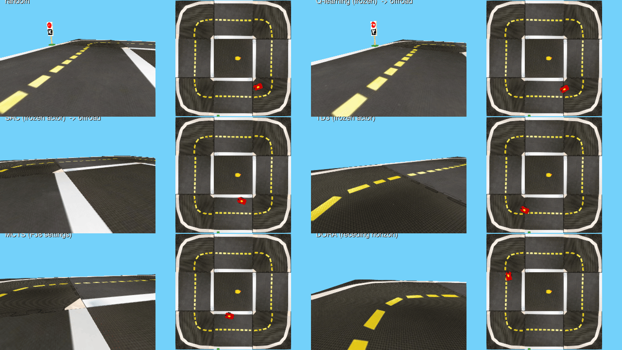
Every built-in driver on the same scenario and spawn (:stop_and_duck_safe, seed 1001), first 40 decisions each, replayed warts included: the frozen tabular policies and the SAC actor leave the road on this spawn, and the segment labels say so. Generated by notebooks/make_solver_gifs.jl. Duckietown environment by the Duckietown Project.
Testing, and reproducing the reported experiments
The recorded results were produced against the frozen configs and trained checkpoints from DuckieMDP, which are not redistributed here. scenario_config gives the right shape of task but not the exact evaluated environment — the reward weights and spawn settings there differ per algorithm.
To run the parity and evaluation test sets, put the reference material beside this package:
parent/
├── Duckietown.jl/      # this repository
└── duckduck/
    └── policies/{q_learning,sarsa,sac,td3}/
        ├── training_config.yaml
        └── policy.npy   (tabular)  |  policy.pt  (SAC/TD3)
Then using Pkg; Pkg.test(). Without it the suite still runs: it skips the 21 reference-dependent files by name and says so, rather than failing or quietly passing.
DDM_SKIP_BENCH=1 skips the planner benchmark (the single most expensive file, ~3.5 of the ~8 minutes) for day-to-day runs — announced, never silent. Leave it unset for release-grade runs.
with the reference     235 test sets, 149 214 assertions
without it             134 test sets,  79 357 assertions
The fixture-based parity layers (FJ2/FJ3) run in both modes — their fixtures are committed — so a referenceless run still re-verifies the dynamics, observers, reward and RNG against recorded reference outputs. Only the sets that need the reference's frozen configs, checkpoints, or its live Python skip themselves.
The authoritative count is the structured report the suite writes to artifacts/fj9/test_report.json, built from the Test result tree rather than by parsing terminal output. tools/suite_summary.sh and the independent tools/suite_summary.py are cross-checks that must agree with it — they disagreed with the reporter on its very first run, which is how a bug in the reporter was caught.
Known limitations
Recorded in full in artifacts/fj9/reproducibility_manifest.json. The ones that most affect how the results should be read:
- The six-solver comparison is not a single comparison. Each solver family was evaluated under its own config, and those differ in reward terms and in spawn distribution — there are two distinct initial-condition sets across the six. Comparisons within (
q_learning,sarsa,mcts) and within (sac,td3,dpw) are properly paired; comparisons across those groups are not. - Parity is not validity. The port is verified against the Python reference. If that model is unrealistic, this reproduces the unrealism faithfully. Nothing here has been checked against a real Duckiebot or a high-fidelity simulator.
- One map, 20 seeds, horizon 150.
goalandtimeoutnever fire in the evaluation: the map defines no goal tile, and the horizon stops episodes well before the environment's own limit. - Planner budgets are small (35–36 iterations). The search results describe behaviour at a low budget, not the algorithms' capability.
- No observation or belief model. See FJ10.